Test the TEXT function!

We will learn something interesting today about a lesser used text function, which is called “TEXT” itself!! Can you ask for an easier name to remember a function? 

Ok, let us get on with the brilliant features available with this function.

Syntax:

=TEXT(value, format)

Where value is the value to convert to text, and format is the format to display the results in.

Format can take one of the following modes – number, date, time, currency, percentage, scientific notation and finally the default text format too.

This function is very rich and powerful with all these different formats and notations, and it would be easier to understand the use of this with some practical examples, than with boring text. 

Look at the following image to understand the concept better.

Example:

Practical tips:

In a real life scenario, you might come across a situation where you get some values in different formats, for instance, the date might get populated as a text and come to you from a database. In such situations, this function can be very handy as you can use a combination of standard set of DATE functions, the LEFT, MID and RIGHT functions to extract the date strings and use the TEXT function to output it in the desired format. 

Similar applications of this function is virtually unlimited and the scope would be as large as your ability to imagine solutions out of this wonderful multipurpose utility function.

Download link:

The example shown above can be downloaded and viewed as well - the sample workbook is stored here for your ready reference - http://sdrv.ms/WiHRNq 

My upcoming book on Excel contains many more such tricks and practical insights into getting Excel work for you. Please take a moment to visit my earlier post to understand details about my new book, and make use of the special offer available now to order it at a discount.

PivotTables – using the Summary functions

Today, let us learn a bit about PivotTables and the convenient assistance they offer us in many ways. This tip is based on a special request from one of my friends P Sreenath, who wanted me to write a few things on Pivots.

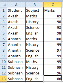
Let us take an example to understand the summary functions better. Consider the following table of student and subject-wise academic performance (data of marks scored):

Now, the school management wants to do a summary analysis by subject and find out the maximum marks scored, the minimum marks scored and the average marks scored, so that they can evaluate the respective subject teachers. 

Since the data is available by student, if we need to get the summary level data by subjects, we must sort the data by subjects and then use the MAX, MIN and AVERAGE worksheet functions on each data range to get the values of maximum, minimum and average scores respectively - see the restructured sample below.

However, there is an easier option available and would be a boon especially when you have a huge number of records to work on. You can forget the manual methods of sorting and applying formula to each selected range of subjects and three different forumulas for each one – in this current example, 4 subjects x 3 functions each = altogether 12 formulas to be setup manually. 

Take recourse to the PivotTables, and let us find an easy solution. Just follow these steps:

Step 1: Select the data range, and click on the PivotTable button on the Insert menu of the Ribbon.

Step 2: Choose your option of New worksheet or existing place in the current worksheet, to get the PivotTable skeleton structure.

Step 3: Drag the Subject field to the Row Labels zone, and drag the Marks field thrice to the Values zone – as shown below:

Step 4: Now click on the first Marks field (“Sum of Marks” in the values zone) and select Value Field settings. In the dialog box, just select the function MAX (instead of the default sum) and click ok.

Step 5: Repeat the process on “Sum of Marks2” – making it MIN and “Sum of Marks3” – making it AVERAGE. Your work is done in a jiffy now. See the summary results below.

Note: 

When you do the average, you will note that there are too many decimals that appear. If you want your worksheet to look clean and without decimals, you can use the value field settings again on that field, select the Number Format button which will bring up the Cell properties dialog box. You can set the field to Number type with zero decimal places there and click OK. Note that the number formatting would be retained on the PivotTable only when you set it through the Value Settings dialog box. If you use the comma button or $ button on the Ribbon to format the cells, the formatting would be lost the next time the Pivot is refreshed. 

The example file is available on Skydrive for you to take a quick online view  - http://sdrv.ms/SsLOOa

Hope you will find this tip useful and handy. I will try to share few more interesting tips on PivotTables in the coming days as well. Would be glad to have your comments on this, and help your friends also to learn a trick or two – share the blog details with them!

My upcoming book on Excel contains many more such tricks and practical insights into getting Excel work for you. Please take a moment to visit my earlier post to understand details about my new book, and make use of the special offer available now to order it at a discount.

An undocumented Excel Function!

I know it could be boring for you to learn about Excel functions, which are available in plenty, and on which Excel Help offers good insight. So, I chose to write about an Excel function today that exists and can be used but on which Excel Help has nothing to say.

You would know that the default way to find difference between two dates is to just use the subtract formula and format the result cell as number. For instance, if Cell A1 contains startdate and A2 contains the enddate, you would enter the formula “=A2-A1” in the result cell, and format it as number to see the days.

Today we are going to learn about a date related function, which is an undocumented Excel function – and is actually a nice utility for computing the difference between two dates. Beauty of this function is that you can get the difference expressed in days, months, years or a combination of any of these. The function is called “DATEDIF” and can produce some unimaginable (positivelyJ ) results, as we would see in the examples that follow.

Formula Syntax:

=DATEDIF(startdate, enddate, interval)

Here, the startdate  and enddate would just be cell references (like A2, A3) which hold the respective dates for which you want to compute the difference. The last parameter, interval, can take one of the following forms (include the quotes):

• “d” to get the result in number of days
• “m” for number of months
• “y” for number of years
• “ym” for number of months (ignoring the year)
• “yd” number of days (ignoring the year)
• “md” number of days (ignoring the month and year)

How it works:

I believe in the saying “A picture speaks a thousand words”. Take a look at the below screenshot which I have constructed for you - it would make things very clear than any number of explanations.

 Deploying a combination formula:

You can obviously make use of this function and deploy a combination trick to get the exact number of years, months and days neatly in your result. See the following picture to understand this – am giving you two variations, the second one would look more neat because I use an additional IF function to take care of the Zero value situation.

That completes the trick for the day. Spread the word around to your friends, if you liked this and find it to be of some use.

My upcoming book on Excel contains many more such tricks and practical insights into getting Excel work for you. Please take a moment to visit my earlier post to understand details about my new book, and make use of the special offer available now to order it at a discount.

My new book - now available at a special price!

Let me admit - am pretty impressed with the number of hits on this relatively new blog, and am very thankful to all of you, readers. As a special measure of thanks, am glad to present you a hard-to-resist offer - an opportunity to order my upcoming book at a whopping discount of 34%.

Yes, you read that right - 34%, but it may not last for too many days. Amazon has opened up this special pricing just for a few days, and if you are interested to get my book, please place your order using the below links, at the earliest.

Here are some details about my new book "Excel for the CFO" - slated for release by 1st November, 2012.

Brief of the title:

Written specifically for finance managers, Excel for the CFO explains the best features of Excel that allow for the automation of regular processes and help reduce the processing time spent on analytics.

The book explores the entire gamut of finance-related functions and is focused on practical approaches to using Excel—including Pivot Tables, Goal Seek, Scenario Builder, and VBA—in problem solving to deliver quality results.

Using case studies across all types of organizations to demonstrate the application of Excel-based automation, the scenarios covered include the automation of financial analysis models, the creation of income statement and balance sheet templates, converting numbers to words for check printing and much more.

Any finance executive who manages the company’s business affairs and makes critical decisions by analyzing data would be directly benefitted by using the tips and techniques presented in this guide.

Pricing:

List Price            : $29.95
Pre-order Price   : $19.77
You Save            : $10.18 (34%)

Amazon Link:
http://www.amazon.com/Excel-CFO-Professionals-P-Hari/dp/1615470115

Incidentally, my other books are available with some good deals. Take a look at these links:
Excel for the CEO - Print edition
Excel for the CEO Ebook (Kindle edition)
Excel for the Small Business Owner (Ebook)

Is it possible to copy Page Setup?

Many of us would have faced this situation - where we take a lot of time to do some specific page setups for a worksheet, and later realise that we did not select the other sheets while doing the setup.

The result? - you would have to do the whole thing all over again, because Excel does not offer a regular menu option to copy the page setup features. We have all sorts of copy-paste, including format painters but when it comes to Page Setup, none of those come to the rescue.

Never mind, trust the experts to always come up with an easy solution. Here we have a simple solution for this complex problem - one of the most appreciated tips from my book "Excel for the CEO".

Problem Statement:

Apply the specific page setup settings for one worksheet to the eight other worksheets in the same workbook.

There is no built-in option to do this in Excel.

Solution steps:

1. What you need to do is very simple – first place your cursor in the sheet that has the page setup you want to use.
2. Now select the sheets where you want to apply the page setup using the mouse cursor while holding down the Ctrl key. 
3. If you are using Excel 2003, select File → Page Setup from the Main menu and just click on OK. 
4. In Excel 2007 & later, Page Setup is available from the Page Layout tab of the Ribbon. Alternate is to select File->Print and then click on the small Page Setup button available under this. 
5. That’s all – your page settings are automatically transferred to the eight new sheets.

Note: Some of the tips shown here are extracts from my book on "Excel for the CEO" - details available at www.mrexcel.com/ceo.shtml. You can also find this in the ebook edition "Excel for the Small Business Owner" available for online ordering at www.mrexcel.com/sbo.shtml

Stop Duplicates!

Let us learn a nice trick today, which can help you to stop duplicates from entering your file.

There are definitely good tools to easily track and report duplicates, like the “Highlight duplicates” feature of the Conditional Formatting group, but we are going to learn a preventive mechanism whereby the duplicate is arrested on entry itself and not as a post mortem exercise.

We shall use the technique of Data Validation to get this done. Given below is a sample scenario and solution:

1.  Select the range in which you want to prevent duplicates – this could be say the range of cells from G1 to G80.
2. From the Ribbon, click on Data->Data Validation (alternate is to use the shortcut keys Alt+D, followed by L)
3. In the first tab of the dialog (Settings), select “Custom” from the “Allow” dropdown box.
4. Now you will get a box to enter formula.
5. In the formula box type this:  =COUNTIF($G$1:$G$80,G1)=1
6. Your sentry tool is now ready for operation, but we will give it some dialogue to display.
7. You have an option to present a customized error message to the users who enter a duplicate value.  To configure this, select the Error Alert tab of the dialog box.
8. In the Title box type "Stop Duplicates!" (or any such thing you like – may be add in your name too to make it very customized)
9. In the Error Message box type "You are trying to enter a duplicate value. Please enter non-duplicates only. " (or any such thing you like)
10. We are all set , just click on the OK button to set the validation on.

The formula used:

If you see the formula used in Step 5 above, it is a simple COUNTIF formula which tells Excel to count how many times the data from the current cell (G1) is included in the range G1:G80.

Excel automatically changes the current cell reference – so if you go to Cell G23 and open the data validation rule again, you will see that the formula would have changed to G23 – like this: =COUNTIF($G$1:$G$80,G23)=1

The formula evaluates and if the count of such values is equal to 1, it means there is no duplicate value. The condition evaluates to TRUE and everything passes through OK. However, if there is a duplicate being entered, the formula evaluates to FALSE (answer not equal to 1), and triggers the error alert, which you have customized above.

Now you have the right tools with you, so just go ahead and stop the dupes ;)

Note: Some of the tips shown here are extracts from my book on "Excel for the CEO" - details available atwww.mrexcel.com/ceo.shtml. You can also find this in the ebook edition "Excel for the Small Business Owner" available for online ordering at www.mrexcel.com/sbo.shtml

Give me a break!

Some of us are so madly in love with Excel that we at times end up using it as a word processing engine, ignoring MS-Word or its equivalents completely.

When you go overboard and start typing longish sentences of text, you would naturally find that Excel treats them with disdain. In other words, you see that your sentence goes a real, long way and it starts at Column A and ends up at say, Column H.

But you are sure to have situations where you prepare a report full of numbers and statistics, accompanied by typical disclaimers or notes at the bottom of the table. If you have to take a nice printout, the disclaimers also should wrap up to the same column size as the data in the above table. So, how do you ensure compliance?

Here are the most obvious choices:

a) Assuming that your data table runs from Column A to Column D and your notes run up to Column H, you will first select the entire set of cells from Column A to D in the notes section, and do a “Merge & Center” (using the button with an “a” in the center – part of the standard formatting toolbar) so that the entire text flows in within the same columns as the data table.

b) Select the merged cells and now click on the “Wrap Text” button in the formatting toolbar to wrap the text nicely in to the merged cells

c) Adjust the row height appropriately so that the entire wrapped text is nicely visible.

Okay, may be this is a fairly simple task. But you can achieve steps a) and b) in one go by selecting the cells, clicking on Ctrl+1 to bring up the formatting dialog box, and choosing “Wrap text” and “Merge cells” checkboxes and clicking Ok.

Now, let’s look at a slightly complex question – what do you do when you want the sentences to be broken at a particular point and flow the next sentence in another line – instead of just continuing and wrapping on?

What I have seen many people do is this – they type the first sentence in one cell/merged cells. They go down to the next row and type the next sentence and so on. This also serves the purpose, but is a hard, round-about way to achieve the result. 

Let’s look at a smart option to get this done.

In comes the keyboard shortcut – Alt+Enter key. When you are entering a stream of sentences, and you want a line break just press this key combination and you will notice that Excel introduces a line break nicely, while allowing you to carry on with your task of typing the next sentence.

This shortcut makes it so simple that you won’t have to cry “Give me a break” ever again! 

Give me a shout if you want any specific topic to be touched upon. I already have a request for Pivot Tables, and would be covering it soon. 

Note: Some of the tips shown here are extracts from my book on "Excel for the CEO" - details available atwww.mrexcel.com/ceo.shtml. You can also find this in the ebook edition "Excel for the Small Business Owner" available for online ordering at www.mrexcel.com/sbo.shtml

The hidden power behind the number keys

We all use the number keys so frequently, and most of us would not have realized the potential behind those numbers.

Wait, am not talking numerology. I mean business with Excel – serious business made simple with some keyboard shortcuts. This shall be the topic for today.

Take a peek at what these number keys could mean for you from tomorrow – if it brings in a positive change, drop in a comment or two and I would be happy to add more in the coming days.

Let’s start with understanding the number keys we are talking about – am including the set of typical keys starting from the tilde character (~) and running up to 0 (zero). These 11 keys offer 22 possible combinations of shortcuts (using Ctrl key and using a combination of Ctrl+Shift keys).

Am giving below a simple table displaying the use of these keys, along with some easy-to-remember tips, which I hope shall soon make you a keyboard addict. That buys you freedom from the mouse!

Table A – 11 possible combinations, using the Ctrl key plus the number keys

Shortcut Keys	Purpose
CTRL + `	Switch view - between normal & formula details view
CTRL + 1	Format Cells dialog box
CTRL + 2	Applies Bold formatting
CTRL + 3	Applies Italic formatting
CTRL + 4	Applies Underline formatting
CTRL + 5	Sets/removes strikeout font in current cell (why not try it on a cell to understand better?)
CTRL + 6	Alternates between hiding objects, displaying objects, and displaying placeholders for objects. (forget it for now, not so useful)
CTRL + 7	Not useful anymore - it was used in earlier versions to display or hide the standard toolbar
CTRL + 8	Displays or hides the outline symbols - useful when you deploy Group/Outline features in your worksheet (forget it again, we will learn it for advanced use later)
CTRL + 9	Hide active row
CTRL + 0	Hide active column

Table B – Another 11 combinations, using the Ctrl and Shift keys plus number keys

Shortcut keys	Purpose
CTRL + SHIFT + `	Format as general number
CTRL + SHIFT + 1	Format as number with 2 decimal places
CTRL + SHIFT + 2	Format as Time - like 07:30 AM (Easy tip to remember - Shift+2 is @ - this character is usually used for time formats in databases)
CTRL + SHIFT + 3	Format as Date - like DD-MMM-YY (Easy tip to remember - Shift+3 is # - this character is usually used for date formats in databases)
CTRL + SHIFT + 4	Format as Currency (Easy tip to remember - Shift+4 is $ - this character is obviously used for currency signs in databases)
CTRL + SHIFT + 5	Format as Percentage (Easy tip to remember - Shift+5 is % - this does not need an explanation)
CTRL + SHIFT + 6	Format as Scientific (Easy tip to remember - Shift+6 is ^ - this applies for Exponential/ scientific formats)
CTRL + SHIFT + 7	Puts a one line border (I can’t think of a tip - find a way to remember!)
CTRL + SHIFT + 8	When you are in a range of cells, pressing this would automatically select the entire range around the current cell - contiguous range
CTRL + SHIFT + 9	Unhide row within the selection
CTRL + SHIFT + 0	Unhide column within the selection

Try your hand at these, and let me know if it helps in simplifying a few things for you. Happy to hear views and comments.

Note: Some of the tips shown here are extracts from my book on "Excel for the CEO" - details available atwww.mrexcel.com/ceo.shtml. You can also find this in the ebook edition "Excel for the Small Business Owner" available for online ordering at www.mrexcel.com/sbo.shtml

Control your numbers - display only thousands or millions

This is something that will come handy for a lot of Finance professionals.

You end up working with thousands of cells with numbers, and each cell has a terrifying 10/12/14  digit number which makes it very difficult to read and comprehend the numbers, leave alone making an analysis.

To overcome this issue, people generally resort to one of these methods:
a) create another sheet where you enter a formula to link up to the original sheet, where they divide the cells by 1000 or 1,000,000 etc and view it in the condensed form.
b) if another backup of the file is available, they use the paste special function (which has got a divide option embedded) to divide the numbers directly by 1000 or 1,000,000 and get the numbers truncated. But the original values would be lost. [Feel free to ask if you need more details on this]

We see that both the methods above can give you the result but are not really a smart way to work. One of the simplest ways to achieve this is to deploy the following trick:
1) Select all your numeric cells.
2) Press Ctrl+1 to bring up the Format Cells dialog box.
3) Now go to the last item in the list (Custom) – and type a zero followed by a comma (0,) under the Type on the right side.
4) Press OK, and you will see that all figures now appear at thousands level. The change has happened only in the display and the cells still retain their original values, as you can witness in the formula bar or by going to the cell and pressing F2 key.
5) If you want it to show only millions, type “0,,” in the custom type box.

Now, does that qualify as a nice tip for the day?

Note: This tip is an extract from my book on "Excel for the CEO" - details available at www.mrexcel.com/ceo.shtml. You can also find this in the ebook edition "Excel for the Small Business Owner" available for online ordering at www.mrexcel.com/sbo.shtml

Welcome to a brand new Excel Blog

Hi,

With great pleasure, I welcome you to my brand new Excel Blog. I have titled it as "Excel with Hari" to share all the little things that I have learnt about Excel in my almost 15 years association with the wonderful tool - MS-Excel.

Here on the blog, I will start posting all the tips, tricks and less-known but more useful functions and utilities related to MS-Excel. Shall try and share something everyday. You can also see a splash of VBA codes here and there.

I welcome you to keep the forum lively with your posts too, and regular feedback.

To start with, I welcome you to take a look at this article on Excel 2010, which I wrote for Que Publishing:
http://www.quepublishing.com/articles/article.aspx?p=1594889

Cheers,
P.K.

See my book on "Excel for the CEO": www.mrexcel.com/ceo.shtml 
Also, my ebook on "Excel for the Small Business Owner": www.mrexcel.com/sbo.shtml